MAIN GUI
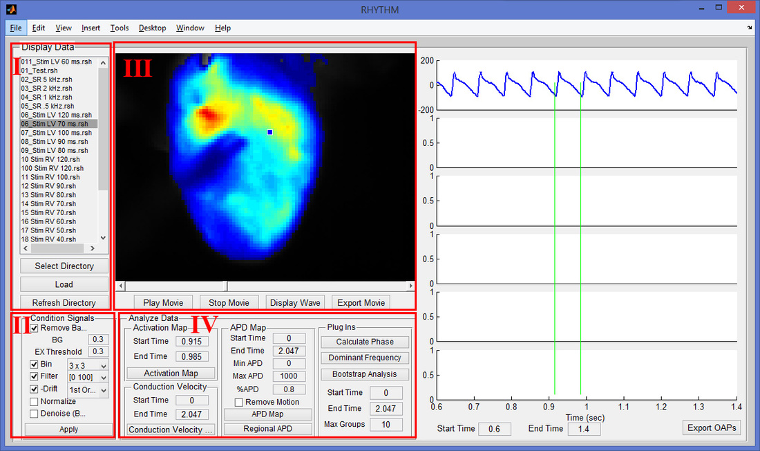
I. Data Loading
- After clicking the “load directory” button, a file browser window opens in which the user can select the target directory.
- After highlighting the desired file, click “load” to load the optical map.
II. Viewing the Optical Map
- This window allows optical maps collected at different time points to be concatenated. By moving the slider, a continuous conduction profile can be played as a movie.
- The “display wave” button allows the user to investigate the conduction profile of a specific point of interest. By placing a pointer to the optical map, the excitation profile of that point would be displayed on the right of the panel.
- The “export movie” button allows the user to export the conduction movie in avi format
III. Signal Processing
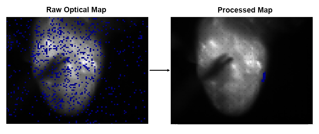
- “Remove background” removes the noise by eliminating the background signal and the excitation signal that are below thresholds specified by the user.
- “Bin” performs a 2D convolution of the data with a matrix of ones. The binning averages each pixel in the matrix with a number of surrounding pixels specified by the user, which can be chosen from a list of 3*3, 5*5 and 7*7.
- “Filter” implements a finite impulse response series of different low and high passbands, including 50Hz, 75Hz, 100Hz, and 150Hz.
- “Drift” removes the drift in the signal by fitting an nth degree polynomial to the data, which is then subtracted from the signal.
IV. Data Analysis
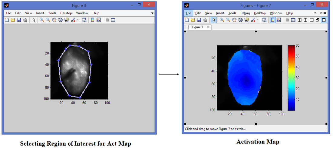
- Activation Map takes the selected period of excitation as input and outputs the time point at which the derivative of electric potential reaches its maximum.
- The activation map prompts the user to select a region of interest and then produce a mask to the original activation map. The “activation map” button produces a map of masked data with background of 0 (background = 0), and a map of masked data without background (background = NaN). The user is able to save the activation map as a .csv file and proceed to further analysis.
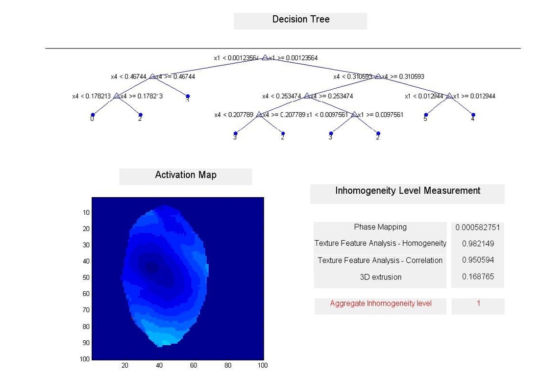
- The inhomogeneity analysis opens a separate window (as shown above) where the decision tree, activation map, and inhomogeneity levels calculated from different methods are presented. The decision tree is pre-determined from a training set of 120 samples and fixd within the software. The activation map is generated in the same manner as in the “activation map” button. The aggregated inhomogeneity level combines all four measurements and gives a weighted value, which is the final prediction of the GUI for the inhomogeneity of the input activation map.
