The software is constituted of four sections as shown in the flow diagram: signal processing, activation map calculation, conduction inhomogeneity quantification and inhomogeneity level determination using machine learning. The details of the algorithms are discussed below.
- Signal Processing
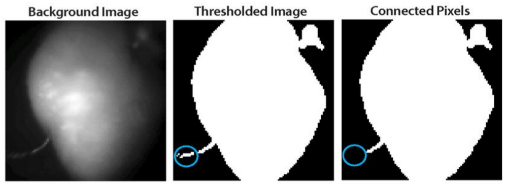
Figure 6 Background removal using thresholding routine [1]
The background removed data is then combined into larger bins to minimize spatial noise and to increase processing efficiency. The default binning factor is 3, which combines 3x3 pixels into a single bin. The binned images are passed into a 100-order finite impulse response (FIR) filter with low pass and high pass threshold frequencies selected by the user. The filter is implemented with Parks-McClellan Remez Exchange Algorithm, which is a standard iterative algorithm that finds the optimal Chebyshev FIR filter. The algorithm minimizes the error in both the pass and stop bands using the Chebyshev approximation theory until both pass and stop bands specifications are met.
The last step in signal processing is drift removal, which corrects for the drift of baseline in the recordings due to photo bleaching or motion [1]. A fourth order polynomial fitting is applied and subtracted from the signal. As shown in Figure 7, a fourth order polynomial (red dash line) is fitted to the optical signal (black) and subtracted to yield a steady baseline signal (blue).
The last step in signal processing is drift removal, which corrects for the drift of baseline in the recordings due to photo bleaching or motion [1]. A fourth order polynomial fitting is applied and subtracted from the signal. As shown in Figure 7, a fourth order polynomial (red dash line) is fitted to the optical signal (black) and subtracted to yield a steady baseline signal (blue).
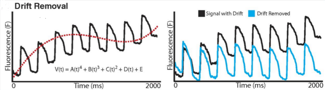
Figure 7 Drift Removal using polynomial fitting algorithm [1]
- Activation map calculation
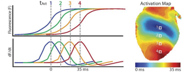
Figure 8 Activation map calculation at 4 different locations on the heart [1]
- Conduction heterogeneity quantification
The first method is phase difference mapping. The time differences of each pixel with its neighboring pixels are calculated, and the maximum time difference is taken as the phase of that pixel. After evaluating the phase on a pixel-by-pixel basis, the output feature inhomogeneity index is calculated as , where is the 95 percentile activation time, is the 5 percentile activation time, and is the median activation time.
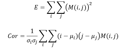
The second method is the gray-scale co-occurrence feature extraction method. Using MATLAB built-in function “graycomatrix”, a gray-level co-occurrence matrix is created. The activation map is first scaled into 8 gray scale levels from 0 to 50 ms, and the frequency of gray scale adjacent to gray level is recorded in the co-occurrence matrix . Then the two inhomogeneity parameters homogeneity (E) and correlation (Cor) are calculated as follow [4]:
The third method is parametric 3D extrusion method modified from the proposed MRI surface area method in [6]. The activation time is treated as the third dimension (height) and the 2D activation map is extruded into a binary 3D object, where 1’s denote voxels inside the object and 0’s denote voxels outside the object. The total surface area is the sum of surface area for each voxel subtracting the surface area that is lost due to neighboring pixels [6]:
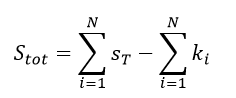
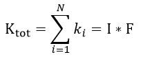
where is the surface area of each voxel, is the total surface area lost for voxel and N is the total number of the voxels. Practically in this project, the total surface area lost is calculated from a convolution of the binary 3D object and a 3x3x3 kernel function F that is 1 on center voxels of each surface and 0 elsewhere:
The final inhomogeneity parameter is the normalized surface area, defined by:
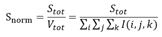
where is the total volume of the object calculated by summing the binary 3D object I.
A 10-fold cross validation is used so that 10 trees are generated with 1/10 of the data set held out, and the average is taken to obtain an unbiased estimate of the true hypothesis. The cross validation is implemented to maintain the optimal balance between the generalization
- Inhomogeneity level determination
A 10-fold cross validation is used so that 10 trees are generated with 1/10 of the data set held out, and the average is taken to obtain an unbiased estimate of the true hypothesis. The cross validation is implemented to maintain the optimal balance between the generalization
and the reliability of the validation
when the validation set needs to be as large as to ensure the validity of the prediction in out of sample data set, it also needs to be as small as to minimize the discrepancy between the held out set (where 1/10 of the samples are excluded) and the whole data set (all the training data included). The cross validation error offers an unbiased estimate of because the is the expectation of all over the input space, which is due to the fact that training set in cross validation offers sufficient data points and a diversity between different data sets.
A reduce-error pruning algorithm is enabled to control overfitting. In this method, the whole data set is split into the training set and validation set . The tree is first grown freely with the training data . After the full tree is obtained, starting from the bottom of the tree, all possible internal nodes are collapsed if it reduces the validation error of the tree, which is generated by applying the tree learned on the held out validation set. This process is repeated recursively up the tree until the error is no longer reduced. This post-pruning technique avoids the risk of missing the best places to prune at one level because the gain at that level is low, but the subsequent levels provide more gains.
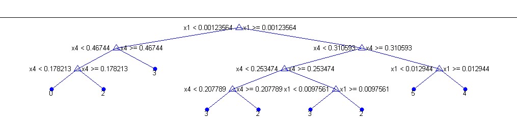
The decision tree, once generated, is stored inside the software package for future use. Every time a new data set is loaded into the software, the four features can be calculated from the data set, and the software is able to give a prediction of the label of the data set by applying the pre-determined decision tree to the four-dimensional input. The software therefore is able to automatically determine the inhomogeneity level using the decision tree algorithm coupled with cross validation and pruning techniques.
A reduce-error pruning algorithm is enabled to control overfitting. In this method, the whole data set is split into the training set and validation set . The tree is first grown freely with the training data . After the full tree is obtained, starting from the bottom of the tree, all possible internal nodes are collapsed if it reduces the validation error of the tree, which is generated by applying the tree learned on the held out validation set. This process is repeated recursively up the tree until the error is no longer reduced. This post-pruning technique avoids the risk of missing the best places to prune at one level because the gain at that level is low, but the subsequent levels provide more gains.
The decision tree, once generated, is stored inside the software package for future use. Every time a new data set is loaded into the software, the four features can be calculated from the data set, and the software is able to give a prediction of the label of the data set by applying the pre-determined decision tree to the four-dimensional input. The software therefore is able to automatically determine the inhomogeneity level using the decision tree algorithm coupled with cross validation and pruning techniques.