Input/Output Overview
The input to the software is a 3D matrix of optical mapping data recorded from the MiCAM ULTIMA (SciMedia, Costa Mesa, CA) imaging system in RealSQLDatabase format (.rsd). Each sub-matrix of the stacked scans is an array of a cardiac optical map at a specific time point, where each pixel represents the fluorescent intensity at a specific location of the heart at that specific time.
The flow chart provided below details how the raw data is processed to yield the final quantification of spatial inhomogeneity. The optical data cube is first loaded in the MATLAB-based RHYTHM GUI for pre-processing to remove image artifacts; these include background removal, binning, filtering, and drift removal (will be discussed in detail below). Filtering and de-noising is followed by the construction of activation maps through manual inspection. The activation maps are the intermediate output which are then used to calculate the phase mapping inhomogeneity index, the homogeneity and correlation parameters of the texture analysis algorithm, as well as the normalized surface area of the 3D extrusion map.
The bottom half of the flow chart represents how the comprehensive model was trained to predict the final heterogeneity score. 120 optical mapping data were used and fed into the RHYTHM software to yield the parameters from the different algorithms, which were recorded as the X values of the training data. During inspection, each data set was also assigned an inhomogeneity level on the scale from 0 to 5. The assigned values were recorded as the Y values (true data labels) of the training data. The MATLAB inbuilt “fitctree” function was used to learn a decision tree on the training data, which was used as the final model in quantifying the inhomogeneity level of optical mapping data. By passing in the inhomogeneity parameters calculated above, the learned decision tree determines the inhomogeneity level of the heart tissue recorded in the input signal on the scale between 0 and 5.
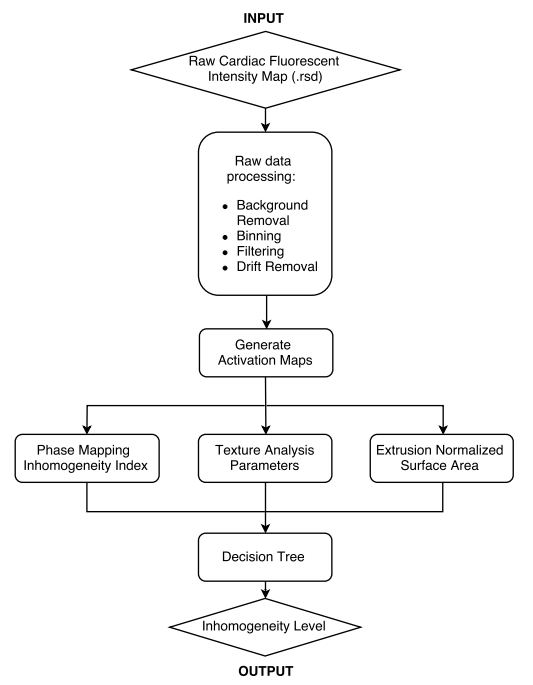
Figure 3 Flow diagram for cardiac optical mapping software
GUI Overview
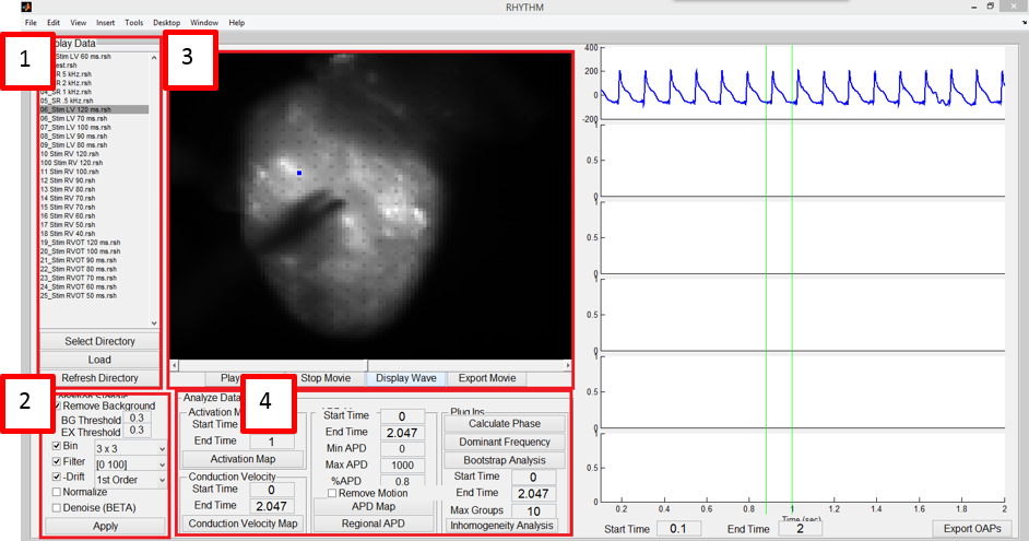
Figure 4 Graphic User Interface for RHTHYM, main window
The final graphical user interface (Figure 4) enables the user to perform a series of actions that start from the raw .rsh files to the determination of the final level of inhomogeneity. The user first loads the data from the data loading panel (1), and then performs background removal, binning, filtering, and drift removal of the data (2). The GUI can then present the signal conduction in the form of a movie and enables the user to give a coarse visual inspection of the inhomogeneity level (3). After selecting a period of conduction, the user can proceed to the inhomogeneity analysis where an aggregate level of inhomogeneity is systematically determined (4).
The separate inhomogeneity level measurement window (Figure 5) displays the built-in decision tree that is used to determine any new data set the user supplies. The four inhomogeneity parameters from phase mapping, texture feature analysis, 3D extrusion are calculated and the final level of inhomogeneity is determined by applying the decision tree on these four features. A detailed user manual is supplied in the Appendix section.
The separate inhomogeneity level measurement window (Figure 5) displays the built-in decision tree that is used to determine any new data set the user supplies. The four inhomogeneity parameters from phase mapping, texture feature analysis, 3D extrusion are calculated and the final level of inhomogeneity is determined by applying the decision tree on these four features. A detailed user manual is supplied in the Appendix section.
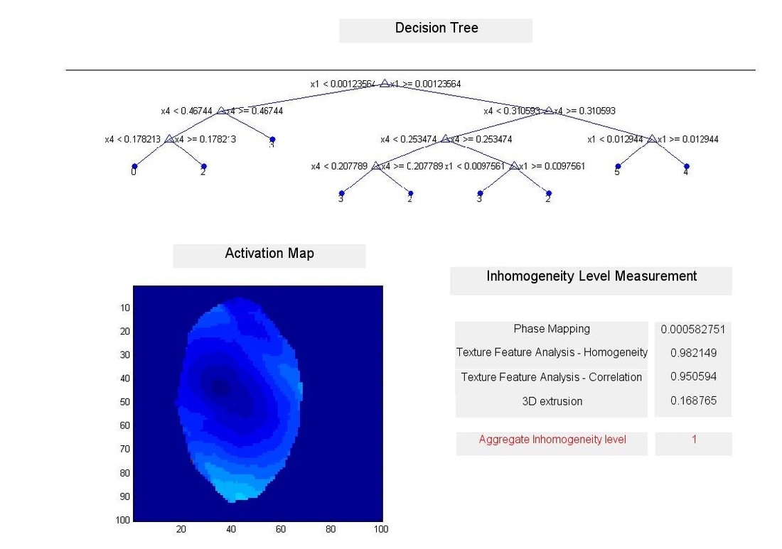
Figure 5 Inhomogeneity Measurement GUI
